DAA Important Questions with Solutions

DAA Important Questions with Answer Diagram and Example(Unit-wise)

Unit 1: Sorting and Analysis

1. Sorting

• Merge Sort
  • Solution: Merge Sort follows the divide and conquer approach. It divides the array into two halves, sorts them recursively, and then merges them in sorted order.
  • Steps:
    1. Divide the unsorted array into two halves.
    2. Recursively sort the two halves.
    3. Merge the sorted halves.
  • Example–
    Input: [38, 27, 43, 3, 9, 82, 10]
    Output: [3, 9, 10, 27, 38, 43, 82]
• Quick Sort
  • Solution: Quick Sort selects a pivot, partitions the array such that elements smaller than the pivot go to the left and larger ones go to the right, and recursively sorts the subarrays.
  • Steps:
    1. Choose a pivot element.
    2. Partition the array around the pivot.
    3. Recursively apply Quick Sort to the subarrays.
  • Example:
    Input: [10, 80, 30, 90, 40, 50, 70]
    Output: [10, 30, 40, 50, 70, 80, 90]

• Heap Sort
  • Solution: Heap Sort uses a binary heap structure to repeatedly extract the maximum element and place it at the end.
  • Steps:
    1. Build a max heap from the array.
    2. Swap the first and last elements.
    3. Reduce heap size and repeat the heapify process.
  • Example:
    Input: [4, 10, 3, 5, 1]
    Output: [1, 3, 4, 5, 10]

2. Recurrence Relation

• Using Master Theorem:
  • Standard form: T(n) = aT(n/b) + f(n)
  • Compare f(n) with n^(log_b(a)) to determine time complexity.
• Using Recursion Tree:
  • Break down the recursive calls to find the overall cost.

3. Growth of Functions

• Big O (O) – Upper Bound
  • Represents the worst-case scenario.
  • It provides an upper limit on the growth rate of a function.
  • It tells us that an algorithm will not take more than a certain amount of time or space.
  • Example: If an algorithm has a time complexity of O(n²), it means the running time will not exceed a quadratic function of the input size.

• Big Theta (Θ) – Tight Bound
  • Represents the average-case scenario.
  • It gives both upper and lower limits, meaning the function grows at a specific rate within constant factors.
  • It describes the exact asymptotic behavior.
  • Example: If an algorithm has a time complexity of Θ(n²), it means the running time grows precisely at a quadratic rate, no more, no less.

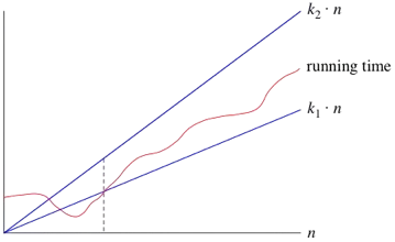
• Big Omega (Ω) – Lower Bound
  • Represents the best-case scenario.
  • It provides a lower limit on the growth rate of a function.
  • It tells us that an algorithm will take at least a certain amount of time or space.
  • Example: If an algorithm has a time complexity of Ω(n²), it means the running time will take at least a quadratic function of the input size.

Unit 2: Advanced Data Structures

1. Red-Black Tree

• A self-balancing binary search tree ensuring O(log n) operations.
• Properties:
  1. Every node is either red or black.
  2. The root is always black.
  3. No two consecutive red nodes.
  4. Every path has the same number of black nodes.
• Example: Insertion and rebalancing steps.

2. Binomial Heap

A binomial heap is a collection of binomial trees that satisfy the heap property.

Structure of Binomial Heap:

• A binomial heap consists of binomial trees, which are recursively defined.
• A binomial tree of order $k$ has:
  • A root node with $k$ child binomial trees of orders $0,1,2,\dots ,k-1$.
  • The number of nodes in a binomial tree of order $k$ is 2k2^k2k.
• The trees are ordered by their sizes, meaning a binomial heap of $n$ nodes will have trees whose orders correspond to the binary representation of $n$.

Operations on Binomial Heap:

1. Insert (O(log n))
   • A new key is inserted as a single-node binomial tree (order 0).
   • The new tree is merged into the existing heap using the merge operation.
   • The process involves combining trees of the same order to maintain the binomial heap structure.
2. Merge (Union) (O(log n))
   • Combines two binomial heaps into one by merging their binomial trees.
   • Trees of the same order are combined recursively, ensuring that no two trees of the same order exist in the final heap.
   • The merge process follows a logic similar to binary addition.
3. Extract Min (O(log n))
   • Finds and removes the smallest key (minimum element) from the heap.
   • The tree containing the minimum element is removed, and its subtrees are separated into a new heap.
   • The new heap is merged back with the remaining heap to restore the binomial heap structure.

Advantages of Binomial Heap:

• Efficient merging of heaps, making it useful in applications requiring frequent merges.
• Supports logarithmic time complexity for key operations like insertion and extraction.
• Well-suited for applications like priority queues and graph algorithms (e.g., Dijkstra’s algorithm).

3. B-Tree

• A balanced multiway search tree used in databases. B-Trees are widely used because they efficiently manage large data while ensuring fast access and updates.

Operations on B-Trees:

1. Search (O(log n))
   • Similar to binary search, the algorithm compares the key with node values and navigates to the correct subtree.
   • Due to the balanced structure, search operations take logarithmic time.
2. Insertion (O(log n))
   • A new key is inserted into the appropriate node while maintaining sorted order.
   • If a node exceeds the maximum allowed keys, it is split, and the middle key is moved up to the parent.
   • Splitting may propagate to the root, increasing the tree height.
3. Deletion (O(log n))
   • A key is removed while ensuring balance.
   • If deletion causes a node to have fewer keys than the minimum required, keys are borrowed or nodes are merged.
   • Similar to insertion, merging can propagate upwards, affecting tree height.

Advantages of B-Trees:

• Fast access: Logarithmic time complexity for search, insert, and delete operations.
• Minimized disk I/O: Optimized for large-scale storage applications.
• Balanced structure: Ensures efficient query performance even with large datasets.
• Scalability: Handles massive amounts of data efficiently.

Applications of B-Trees:

• Database indexing (e.g., MySQL, PostgreSQL).
• File systems (e.g., NTFS, ext4).
• Storage systems requiring efficient read/write operations.

4. Fibonacci Heap (Less Important)

• A heap supporting fast decrease-key operations.
• Operations: Insert, Union, Extract Min.

Operations:

1. Insert (O(1) amortized): Adds a new element to the root list without restructuring.
2. Union (O(1) amortized): Merges two heaps by combining their root lists.
3. Extract Min (O(log n) amortized): Removes the smallest element and consolidates trees.
4. Decrease-Key (O(1) amortized): Reduces a node’s key and moves it to the root list if needed.
5. Delete (O(log n) amortized): Decreases a key to negative infinity and extracts the minimum.

Advantages:

• Fast decrease-key operation, useful in graph algorithms.
• Efficient for frequent priority updates.

Disadvantages:

• Complex implementation and higher constant factors.

Applications:

Dijkstra’s algorithm, network optimization, and priority scheduling.

Unit 3: Optimization Problems

1. Convex Hull and Searching

• Convex Hull algorithms like Graham’s scan for finding the outer boundary. The Graham’s Scan algorithm finds it in $O(n\log n)$ time by:
  1. Find the pivot: Select the point with the lowest y-coordinate (or lowest x if y’s are tied).
  2. Sort points by polar angle relative to the pivot.
  3. Construct the hull: Use a stack to process the points, keeping only those that form a counter-clockwise turn with the last two points.
  4. Time Complexity: $O(n\log n)$.

• Example:

  For points $(0,0),(2,1),(1,3),(3,2),(4,0)$, the convex hull is:

  $$(0,0),(4,0),(3,2),(1,3)$$

  Applications:

  • Computer graphics, collision detection, robotics, GIS.

2. Knapsack Problem

• Problem: Given a set of items with weights and profits, find the maximum profit without exceeding a weight limit.
• Dynamic Programming Solution:
  1. Use a 2D table where each entry represents the maximum profit for a given weight and item set.
  2. For each item, decide whether to include it or exclude it based on the maximum profit achievable.
  • Time Complexity: $O(nW)$, where $n$ is the number of items and $W$ is the weight capacity.

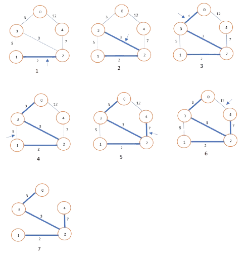
3. Prim’s and Kruskal’s Algorithm

• Prim’s Algorithm:
  1. Start from an arbitrary node, adding the minimum weight edge to grow the MST.
  2. Use a priority queue to select the next closest vertex.
  • Time Complexity: $O(E\log V)$, where $E$ is edges and $V$ is vertices.

• Kruskal’s Algorithm:
  1. Sort all edges in ascending weight order.
  2. Use a union-find structure to add edges to the MST, ensuring no cycles are formed.
  • Time Complexity: $O(E\log E)$, dominated by sorting edges.

4. Dijkstra’s Algorithm

• Problem: Find the shortest path in a graph with non-negative edge weights.

• Greedy Approach:
  1. Use a priority queue to always pick the node with the smallest tentative distance.
  2. Update distances to neighbors and repeat until all nodes are processed.
  • Time Complexity: $O((V+E)\log V)$, where $V$ is vertices and $E$ is edges.

5. Bellman-Ford Algorithm (Less Important)

• Problem: Find the shortest path in graphs with negative weights, and detect negative weight cycles.
• Dynamic Programming Approach:
  1. Relax all edges repeatedly up to $V-1$ times (where $V$ is the number of vertices).
  2. Check for negative cycles by seeing if further relaxation is possible.
  • Time Complexity: $O(VE)$, where $V$ is vertices and $E$ is edges.

Unit 4: Advanced Algorithms

1. Knapsack (Dynamic Programming)

• Problem: Maximize profit without exceeding a weight limit.
• Dynamic Programming Solution:
  1. Define a 2D DP table dp[i][w], where i is the number of items and w is the weight.
  2. For each item, choose between including or excluding it based on whether it increases the profit without exceeding the weight.
  3. Fill the table iteratively based on previous results.
  • Time Complexity: $O(nW)$, where $n$ is the number of items and $W$ is the weight capacity.

2. Warshall’s and Floyd’s Algorithm

• Warshall’s Algorithm: Computes transitive closure of a directed graph, determining if there is a path between every pair of vertices.
  • Time Complexity: O(V3)O(V^3)O(V3), where $V$ is the number of vertices.
• Floyd-Warshall Algorithm: Computes the all-pairs shortest paths for a graph with both positive and negative weights.
  1. Iteratively update the shortest paths between every pair of vertices using an intermediate vertex.
  2. If a shorter path is found via an intermediate vertex, update the path.
  • Time Complexity: O(V3)O(V^3)O(V3), where $V$ is the number of vertices.

3. Backtracking

• Method: Explore all possible solutions recursively and backtrack when a solution path is invalid or incomplete.
  1. Start with an empty solution and attempt to extend it by adding one element at a time.
  2. If the current solution doesn’t lead to a valid complete solution, backtrack and try another option.
  • Applications: Solving combinatorial problems like Sudoku, N-Queen, or the Hamiltonian path.
  • Time Complexity: Depends on the problem; often exponential in nature.

4. Travelling Salesman Problem (TSP)

• Problem: Find the shortest possible route that visits every city once and returns to the origin.
• Dynamic Programming Solution (Held-Karp Algorithm):
  1. Use a DP table to store the shortest path covering each subset of cities and the last city in the subset.
  2. Solve recursively by considering each possible next city and updating the minimum cost.
  • Time Complexity: O(n22n)O(n^2 2^n)O(n22n), where $n$ is the number of cities.

• Approximation:
  1. Greedy Heuristic: Start from an arbitrary city, always travel to the nearest unvisited city.
  2. Christofides’ Algorithm: Provides a 3/2 approximation for metric TSP (triangle inequality holds).
  • Time Complexity for Approximation: O(n2)O(n^2)O(n2).

5. N-Queen Problem

• Problem: Place N queens on an N×N chessboard such that no two queens threaten each other (no same row, column, or diagonal).
• Backtracking Solution:
  1. Place queens row by row, checking for conflicts in columns and diagonals.
  2. Backtrack when a placement leads to a conflict.
  3. Continue until all queens are placed safely.
  • Time Complexity: Typically $O(N!)$ due to the factorial number of possible placements.